Creating a Lower Limb Panoramic X-ray

Measurement of knee alignment is useful for diagnosis of arthritic conditions and for planning and evaluation of surgical interventions. Alignment is measured by the hip-knee-ankle ($HKA$) angle in standing, load bearing, x-ray images. The angle is defined by the femoral and tibial mechanical axes. The femoral axis is defined by the center of the femur head and the mid condylar point. The tibial axis is defined by the center of the tibial plateau to the center of the tibial plafond.

Hip-Knee-Ankle angle defined by the femoral mechanical axis (solid red line with dashed extension), and tibial mechanical axis (solid blue line).

The three stances defined by the $HKA$ angle are:

1. Neutral alignment, $HKA=0^o$.
2. Varus, bow-legged, $HKA<0^o$.
3. Valgus, knock-kneed, $HKA>0^o$.

For additional information see:

1. T. D. Cooke et al., "Frontal plane knee alignment: a call for standardized measurement", J Rheumatol. 2007.
2. A. F. Kamath et al., "What is Varus or Valgus Knee Alignment?: A Call for a Uniform Radiographic Classification", Clin Orthop Relat Res. 2010.

For a robust estimate of the $HKA$ angle we would like to use a single image that contains the anatomy from the femoral head down to the ankle. Acquisition of such an image with standard x-ray imaging devices is not possible. It is achievable by acquiring multiple partially overlapping images and aligning, registering, them to the same coordinate system. The subject of this notebook.

This notebook is based in part on the work described in: "A marker-free registration method for standing X-ray panorama reconstruction for hip-knee-ankle axis deformity assessment", Y. K. Ben-Zikri, Z. Yaniv, K. Baum, C. A. Linte, Computer Methods in Biomechanics and Biomedical Engineering: Imaging & Visualization, DOI:10.1080/21681163.2018.1537859.

import SimpleITK as sitk
import numpy as np
import os.path
import copy

%matplotlib notebook
import gui
import matplotlib.pyplot as plt

#utility method that either downloads data from the Girder repository or
#if already downloaded returns the file name for reading from disk (cached data)
%run update_path_to_download_script
from downloaddata import fetch_data as fdata

Loading data

# Fetch all of the data associated with this example.
data_directory = os.path.dirname(fdata("leg_panorama/readme.txt"))

hip_image =  sitk.ReadImage(os.path.join(data_directory,'hip.mha'))
knee_image =  sitk.ReadImage(os.path.join(data_directory,'knee.mha'))
ankle_image =  sitk.ReadImage(os.path.join(data_directory,'ankle.mha'))

gui.multi_image_display2D([hip_image, knee_image, ankle_image], figure_size=(10,4));

Fetching leg_panorama/readme.txt

Getting to know your data

As our goal is to register the images we need to identify an appropriate similarity metric and transformation type.

Similarity metric

Given that we are using the same device to acquire multiple partially overlapping images, we would expect that the intensities for the same anatomical structures are the same in all images. We start by visually inspecting the images displayed above. If you hover the cursor over the images you will see the intensity value on the bottom right.

We next plot the histogram for one of the images.

intensity_profile_image = knee_image
fig = plt.figure()
plt.hist(sitk.GetArrayViewFromImage(intensity_profile_image).flatten(),bins=100);

Notice that the image has a high dynamic range which is mapped to a low dynamic range when displayed, so we cannot observe all underlying intensity variations. Ideally intensity variations in x-ray images only occur when there are variations in the imaged object. In practice, we can observe non uniform intensities due to the structure of the x-ray device (e.g. absorption of photons by the x-ray anode,known as the heel effect).

In the next code cells we define a rectangular region of interest (use left mouse button, click and drag to define) in an area that is expected to have uniform intensity values (air) and plot the mean intensity per row. You can readily notice that there are intensity variations in what is expected to be a uniform region.

# The ROI we specify is in a region that is expected to have uniform intensities.
# You can clear this ROI and specify your own in the GUI below.
roi_list = [((396, 436), (52, 1057))]
roi_gui = gui.ROIDataAquisition(intensity_profile_image, figure_size=(8,4))
roi_gui.set_rois(roi_list)

# Get the region of interest (first entry in the list of ROIs)
roi = roi_gui.get_rois()[0]
intensities = sitk.GetArrayFromImage(intensity_profile_image[roi[0][0]:roi[0][1], roi[1][0]:roi[1][1]])

fig, axes = plt.subplots(1, 2, sharey=True)
fig.suptitle('intensity variations (mean row value)')
axes[0].imshow(intensities, cmap=plt.cm.Greys_r)
axes[0].set_axis_off()
axes[1].plot(intensities.mean(axis=1), range(intensities.shape[0]))
axes[1].get_yaxis().set_visible(False)
axes[1].tick_params(axis='x', rotation=-90)
plt.box(on=None)

Given our observations above, we will use correlation as our similarity measure and not mean squares.

Transformation type

In general, the x-ray machine is modeled as a pinhole camera, with our images acquired using a fronto-parallel setup and the camera undergoing translation. This simplifies the general model from a homography transformation between images to a planar translation. For a detailed derivation see Z. Yaniv, L. Joskowicz, "Long Bone Panoramas from Fluoroscopic X-ray Images", IEEE Trans Med Imaging. 2004.

While our transformation type is translation, looking at multiple triplets of images we observed that the size of overlapping regions, expected translations, has significant variability. Consequentially, we will use a heuristic exploration-exploitation approach to improve the robustness of our registration approach.

Registration - Exploration Step

As image overlap has considerable variation we will use the ExhaustiveOptimizer to obtain several starting points, our exploration step. We then start a standard registration using these initial transformation estimates, our exploitation step. Finally we select the best transformation from the exploitation step.

class Evaluate2DTranslationCorrelation:
    '''
    Class for evaluating the correlation value for a given set of 
    2D translations between two images. The general relationship between
    the fixed and moving images is assumed (fixed is "below" the moving).
    We use the Exhaustive optimizer to sample the possible set of translations
    and an observer to tabulate the results.
    
    In this class we abuse the Python dictionary by using a float
    value as the key. This is a unique situation in which the floating
    values are fixed (not resulting from various computations) so that we 
    can compare them for exact equality. This means they have the 
    same hash value in the dictionary.
    '''
    def __init__(self, metric_sampling_percentage, min_row_overlap, 
                 max_row_overlap, column_overlap, dx_step_num,
                 dy_step_num):
        '''
        Args:
            metric_sampling_percentage: Percentage of samples to use
                                        when computing correlation.
            min_row_overlap: Minimal number of rows that overlap between 
                             the two images.
            max_row_overlap: Maximal number of rows that overlap between 
                             the two images.
            column_overlap: Maximal translation in columns either in positive
                            and negative direction.
            dx_step_num: Number of samples in parameter space for translation along 
                         the x axis is 2*dx_step_num+1.
            dy_step_num: Number of samples in parameter space for translation along 
                         the y axis is 2*dy_step_num+1.
                             
        '''
        self._registration_values_dict = {}
        self.X = None
        self.Y = None
        self.C = None
        self._metric_sampling_percentage = metric_sampling_percentage
        self._min_row_overlap = min_row_overlap
        self._max_row_overlap = max_row_overlap
        self._column_overlap = column_overlap
        self._dx_step_num = dx_step_num
        self._dy_step_num = dy_step_num
      
    def _start_observer(self):
        self._registration_values_dict = {}
        self.X = None
        self.Y = None
        self.C = None
        

    def _iteration_observer(self, registration_method):
        x,y = registration_method.GetOptimizerPosition()
        if y in self._registration_values_dict.keys():
            self._registration_values_dict[y].append((x,registration_method.GetMetricValue()))
        else:
            self._registration_values_dict[y]= [(x,registration_method.GetMetricValue())]

            
    def evaluate(self, fixed_image, moving_image):
        '''
        Assume the fixed image is lower than the moving image (e.g. fixed=knee, moving=hip).
        The transformations map points in the fixed_image to the moving_image.
        Args:
            fixed_image: Image to use as fixed image in the registration.
            moving_image: Image to use as moving image in the registration.
        '''
        minimal_overlap = np.array(moving_image.TransformContinuousIndexToPhysicalPoint((-self._column_overlap, moving_image.GetHeight()-self._min_row_overlap))) - np.array(fixed_image.GetOrigin())
        maximal_overlap = np.array(moving_image.TransformContinuousIndexToPhysicalPoint((self._column_overlap, moving_image.GetHeight()-self._max_row_overlap))) - np.array(fixed_image.GetOrigin())
        transform = sitk.TranslationTransform(2,((maximal_overlap[0]+minimal_overlap[0])/2.0,(maximal_overlap[1]+minimal_overlap[1])/2.0))
    
        # Total number of evaluations, translations along the y axis in both directions around the initial
        # value is 2*dy_step_num+1.
        dy_step_length = (maximal_overlap[1] - minimal_overlap[1])/(2*self._dy_step_num)
        dx_step_length = (maximal_overlap[0] - minimal_overlap[0])/(2*self._dx_step_num)
        step_length = dx_step_length
        parameter_scales = [1, dy_step_length/dx_step_length]

        registration_method = sitk.ImageRegistrationMethod()
        registration_method.SetMetricAsCorrelation()
        registration_method.SetMetricSamplingStrategy(registration_method.RANDOM)
        registration_method.SetMetricSamplingPercentage(self._metric_sampling_percentage)   
        registration_method.SetInitialTransform(transform, inPlace=True)
        registration_method.SetOptimizerAsExhaustive(numberOfSteps=[self._dx_step_num, self._dy_step_num], 
                                                     stepLength = step_length)
        registration_method.SetOptimizerScales(parameter_scales)

        registration_method.AddCommand(sitk.sitkIterationEvent, lambda: self._iteration_observer(registration_method))
        registration_method.AddCommand(sitk.sitkStartEvent, self._start_observer )
        registration_method.Execute(fixed_image, moving_image)

        # Convert the data obtained by the observer to three numpy arrays X,Y,C            
        x_lists = []
        val_lists = []
        for k in self._registration_values_dict.keys():
            x_list, val_list = zip(*(sorted(self._registration_values_dict[k])))
            x_lists.append(x_list)
            val_lists.append(val_list)
    
        self.X = np.array(x_lists)
        self.C = np.array(val_lists)
        self.Y = np.array([list(self._registration_values_dict.keys()),]*self.X.shape[1]).transpose()

    def get_raw_data(self):
        '''
        Get the raw data, the translations and corresponding correlation values.
        Returns:
            A tuple of three numpy arrays (X,Y,C) where (X[i], Y[i]) are the translation
            and C[i] is the correlation value for that translation.
        '''
        return (np.copy(self.X), np.copy(self.Y), np.copy(self.C)) 
    
    
    def get_candidates(self, num_candidates, correlation_threshold, nms_radius=2):
        '''
        Get the best (most correlated, minimal correlation value) transformations
        from the sample set.
        Args:
            num_candidates: Maximal number of candidates to return.
            correlation_threshold: Minimal correlation value required for returning
                                   a candidate.
            nms_radius: Non-Minima (the optimizer is negating the correlation) suppression 
                        region around the local minimum.
        Returns: 
            List of tuples containing (transform, correlation). The order of the transformations
            in the list is based on the correlation value (best correlation is entry zero).            
        '''
        candidates = []
        _C = np.copy(self.C)
        done = num_candidates-len(candidates)<=0
        while not done:
            min_index = np.unravel_index(_C.argmin(), _C.shape)
            if(-_C[min_index]<correlation_threshold):
                done = True
            else:
                candidates.append((sitk.TranslationTransform(2, (self.X[min_index], self.Y[min_index])), self.C[min_index]))
                # None-minima suppression in the region around our minimum
                start_nms = np.maximum(np.array(min_index) - nms_radius, np.array([0,0]))
                # for the end coordinate we add nms_radius+1 because the slicing operator _C[], 
                # excludes the end
                end_nms = np.minimum(np.array(min_index) + nms_radius + 1, np.array(_C.shape))
                _C[start_nms[0]:end_nms[0], start_nms[1]:end_nms[1]] = 0
                done = num_candidates-len(candidates)<=0 
        return candidates
    

def create_images_in_shared_coordinate_system(image_transform_list):
    '''
    Resample a set of images onto the same region in space (the bounding)
    box of all images.
    Args:
        image_transform_list: A list of tuples each containing a transformation and an image. The transformations map the
                              images to a shared coordinate system.
    Returns:
        list of images: All images are resampled into the same coordinate system and the bounding box of all images is
                        used to define the new image extent onto which the originals are resampled. The background value
                        for the resampled images is set to 0.
    '''
    pnt_list = []
    for image, transform in image_transform_list:
        pnt_list.append(transform.TransformPoint(image.GetOrigin()))
        pnt_list.append(transform.TransformPoint(image.TransformIndexToPhysicalPoint((image.GetWidth()-1, image.GetHeight()-1))))
 
    max_coordinates = np.max(pnt_list, axis=0)
    min_coordinates = np.min(pnt_list, axis=0)
    
    # We assume the spacing for all original images is the same and we keep it.
    output_spacing = image_transform_list[0][0].GetSpacing()
    # We assume the pixel type for all images is the same and we keep it.
    output_pixelID = image_transform_list[0][0].GetPixelID()
    # We assume the direction for all images is the same and we keep it.
    output_direction = image_transform_list[0][0].GetDirection()
    output_width = int(np.round((max_coordinates[0] - min_coordinates[0])/output_spacing[0]))
    output_height = int(np.round((max_coordinates[1] - min_coordinates[1])/output_spacing[1]))
    output_origin = (min_coordinates[0], min_coordinates[1])
            
    images_in_shared_coordinate_system = []
    for image, transform in image_transform_list:
        images_in_shared_coordinate_system.append(sitk.Resample(image, (output_width, output_height), transform.GetInverse(), sitk.sitkLinear, 
                                                                output_origin, output_spacing, output_direction, 0.0, output_pixelID))
    return images_in_shared_coordinate_system


def composite_images_alpha_blending(images_in_shared_coordinate_system, alpha=0.5):
    '''
    Composite a list of images sharing the same extent (size, origin, spacing, direction cosine).
    Args: 
        images_in_shared_coordinate_system: A list of images sharing the same meta-information (origin, size, spacing, direction cosine).
        We assume zero denotes background.
    Returns:
        SimpleITK image with pixel type sitkFloat32: alpha blending of the images.
    
    '''
    # Composite all of the images using alpha blending where there is overlap between two images, otherwise
    # just paste the image values into the composite image. We assume that at most two images overlap.
    composite_image = sitk.Cast(images_in_shared_coordinate_system[0], sitk.sitkFloat32)
    for img in images_in_shared_coordinate_system[1:]:
        current_image = sitk.Cast(img, sitk.sitkFloat32)
        mask1 = sitk.Cast(composite_image != 0, sitk.sitkFloat32)
        mask2 = sitk.Cast(current_image != 0, sitk.sitkFloat32)
        intersection_mask = mask1*mask2
        composite_image = alpha*intersection_mask*composite_image + (1-alpha)*intersection_mask*current_image + \
                          (mask1-intersection_mask)*composite_image + \
                          (mask2-intersection_mask)*current_image 
    return composite_image

We start by performing our exploration step, obtaining multiple starting point candidates.

Below we also plot the similarity metric surfaces and minimal values.

metric_sampling_percentage=0.2
min_row_overlap=20 
max_row_overlap=0.5*hip_image.GetHeight()
column_overlap=0.2*hip_image.GetWidth()
dx_step_num=4
dy_step_num=10

initializer = Evaluate2DTranslationCorrelation(metric_sampling_percentage,
                                               min_row_overlap, 
                                               max_row_overlap, 
                                               column_overlap, 
                                               dx_step_num,
                                               dy_step_num)

# Get potential starting points for the knee-hip images.
initializer.evaluate(fixed_image=sitk.Cast(knee_image, sitk.sitkFloat32), moving_image=sitk.Cast(hip_image, sitk.sitkFloat32))
plotting_data = [('knee 2 hip', initializer.get_raw_data())]
k2h_candidates = initializer.get_candidates(num_candidates=4, correlation_threshold=0.5)

# Get potential starting points for the ankle-knee images.
initializer.evaluate(fixed_image=sitk.Cast(ankle_image, sitk.sitkFloat32), moving_image=sitk.Cast(knee_image, sitk.sitkFloat32))
plotting_data.append(('ankle 2 knee', initializer.get_raw_data()))
a2k_candidates = initializer.get_candidates(num_candidates=4, correlation_threshold=0.5)

# Plot the similarity metric terrain and mark the minimum with a red sphere.
from mpl_toolkits.mplot3d import Axes3D 
fig = plt.figure(figsize=(10,4))
for i, plot_data in enumerate(plotting_data,1):
    ax = fig.add_subplot(1,2,i, projection='3d')
    ax.plot_surface(*(plot_data[1]))
    ax.set_xlabel('x translation')     
    ax.set_ylabel('y translation')
    ax.set_zlabel('negative correlation')
    ax.set_title(plot_data[0])
    min_index = np.unravel_index((plot_data[1])[2].argmin(), (plot_data[1])[2].shape)
    ax.scatter((plot_data[1])[0][min_index], (plot_data[1])[1][min_index], (plot_data[1])[2][min_index],
               marker='o', color='red');

# We will use the hip image coordinate system as the common coordinate system
# and visualize the results with the transformations corresponding to the best 
# similarity metric values.
knee2hip_transform = k2h_candidates[0][0]
ankle2knee_transform = a2k_candidates[0][0]
ankle2hip_transform = sitk.Transform(knee2hip_transform)
ankle2hip_transform.AddTransform(ankle2knee_transform)
image_transform_list = [(hip_image, sitk.TranslationTransform(2)),
                        (knee_image, knee2hip_transform),
                        (ankle_image, ankle2hip_transform)]
composite_image = composite_images_alpha_blending(create_images_in_shared_coordinate_system(image_transform_list))

gui.multi_image_display2D([composite_image], figure_size=(4,8));
print('knee2hip_correlation: {0:.2f}'.format(k2h_candidates[0][1]))
print('ankle2hip_correlation: {0:.2f}'.format(a2k_candidates[0][1]))

knee2hip_correlation: -0.84
ankle2hip_correlation: -0.99

Registration - Exploration Step

Now that we have a set of good (from a similarity metric standpoint) initial estimates for the transformation we will refine them using standard GradientDescent based registration. The final transformations are those that correspond to the best similarity metric values.

def final_registration(fixed_image, moving_image, initial_mutable_transformations):
    '''
    Register the two images using multiple starting transformations.
    Args:
        fixed_image (SimpleITK image): Estimated transformation maps points from this image to the
                                       moving_image.
        moving_image (SimpleITK image): Estimated transformation maps points from the fixed image to 
                                        this image.                                        
       initial_mutable_transformations (iterable, list like): Set of initial transformations, these will
                                                              be modified in place.
    '''    
    registration_method = sitk.ImageRegistrationMethod()
    registration_method.SetMetricAsCorrelation()
    registration_method.SetMetricSamplingStrategy(registration_method.RANDOM)
    registration_method.SetMetricSamplingPercentage(0.2)   
    registration_method.SetOptimizerAsGradientDescent(learningRate=1.0, numberOfIterations=200)     
    registration_method.SetOptimizerScalesFromPhysicalShift() 
    
    def reg(transform):
        registration_method.SetInitialTransform(transform)
        registration_method.Execute(fixed_image, moving_image)
        return registration_method.GetMetricValue()
    
    final_values = [reg(transform) for transform in initial_mutable_transformations]     
    return list(zip(initial_mutable_transformations, final_values))
    

# Copy the initial transformations for use in the final registration
initial_transformation_list_k2h = [sitk.TranslationTransform(t) for t, corr in k2h_candidates]
initial_transformation_list_a2k = [sitk.TranslationTransform(t) for t, corr in a2k_candidates]

# Perform the final registration
k2h_final = final_registration(fixed_image=sitk.Cast(knee_image, sitk.sitkFloat32), 
                                moving_image=sitk.Cast(hip_image, sitk.sitkFloat32), 
                                initial_mutable_transformations=initial_transformation_list_k2h)
a2k_final = final_registration(fixed_image=sitk.Cast(ankle_image, sitk.sitkFloat32), 
                                moving_image=sitk.Cast(knee_image, sitk.sitkFloat32), 
                                initial_mutable_transformations=initial_transformation_list_a2k)

knee2hip = min(k2h_final, key=lambda x: x[1])
knee2hip_transform = knee2hip[0]

ankle2knee = min(a2k_final, key=lambda x: x[1])
ankle2hip_transform = sitk.Transform(knee2hip_transform)
ankle2hip_transform.AddTransform(ankle2knee[0])

image_transform_list = [(hip_image, sitk.TranslationTransform(2)),
                        (knee_image, knee2hip_transform),
                        (ankle_image, ankle2hip_transform)]
composite_image = composite_images_alpha_blending(create_images_in_shared_coordinate_system(image_transform_list))

gui.multi_image_display2D([composite_image], figure_size=(4,8));
print('knee2hip_correlation: {0:.2f}'.format(knee2hip[1]))
print('ankle2hip_correlation: {0:.2f}'.format(ankle2knee[1]))

knee2hip_correlation: -0.92
ankle2hip_correlation: -0.99

Additional food for thought

1. Does the best final transformation correspond to the best initial one?
2. Find the optimal parameter space sampling for the exploration stage (consider both time and accuracy).

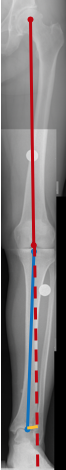
Measure the angle

Start from the top and mark the points in the following order:

1. Femoral head.
2. Femoral mid-condylar point.
3. Center of tibial spines notch.
4. Center of the tibial plafond.

measurement_gui = gui.PointDataAquisition(composite_image);

points_top_to_bottom = measurement_gui.get_points()
if len(points_top_to_bottom) == 4:
    femoral_axis = np.array(points_top_to_bottom[1]) - np.array(points_top_to_bottom[0])
    tibial_axis = np.array(points_top_to_bottom[3]) - np.array(points_top_to_bottom[2])
    angle = np.arctan2(tibial_axis[1], tibial_axis[0]) - np.arctan2(femoral_axis[1], femoral_axis[0])

    print('Angle is (degrees): {0}'.format(np.degrees(angle)))